Introduction

As a teaching assistant this semester for the Intro to Quantum Computing course at UMich, I’ve enjoyed helping students learn the foundations of quantum error correction through detailed coding projects and homeworks. The final project in this class focuses on implementing error correction with fault tolerance—two concepts that many students initially assume are the same. My intention with this blog post is twofold:

To clear up this common misconception with a very high-level overview:
Error Correction is not the same as Fault Tolerance.
To answer the questions students frequently ask, such as:
What’s error correction? What’s fault tolerance? Why is it hard to implement both in practice? What challenges show up at the hardware and system level?

In undergrad when I first looked these answers up online, I often ran into pages of dense math, intimidating terminology, and complicated figures when all I really wanted was an intuitive big-picture explanation before diving deep. So in this post, I aim to give exactly that: a short, high-level intro to both ideas by abstracting away the complicated details.

In short, error correction and fault tolerance go hand-in-hand, but they’re not the same. In fact, you can implement error correction without fault tolerance (though this would be a terrible idea on today’s noisy devices). Alright—let’s jump in.

What’s Error Correction?

Quantum computers do exist—but they are extremely error-prone. The quantum version of the classical bit—called a qubit—is nowhere near perfect. You can imagine a qubit as an electron that can be in one of two states (spin-up or spin-down).

In classical computers, thermal agitation, radiation, voltage fluctuations, and other physical effects can cause bit-flips—but they are astronomically rare. For context, a transistor in a modern laptop experiences such a random bit-flip roughly once every 10⁹ years, corresponding to around 1 error per 10²⁴ operations.

On the other hand, qubits are extremely noisy. The best devices today have qubits that fail once per 10⁴ operations—far worse than the error rates of your laptop’s transistors. So why can’t we just keep improving qubit hardware until these errors disappear?

While hardware advances and shielding can suppress noise, there is a fundamental limit to how reliable a bare physical qubit can be. This motivates a complementary solution: Detect which qubits have errored, and correct them as they happen. This is the essence of quantum error correction.

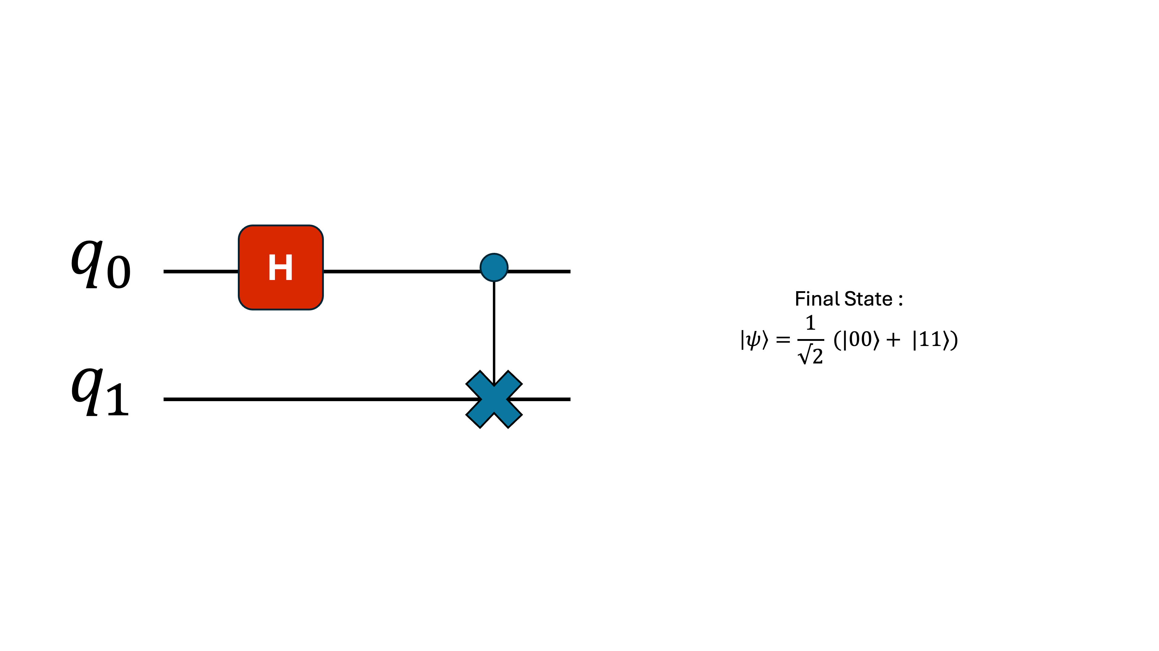
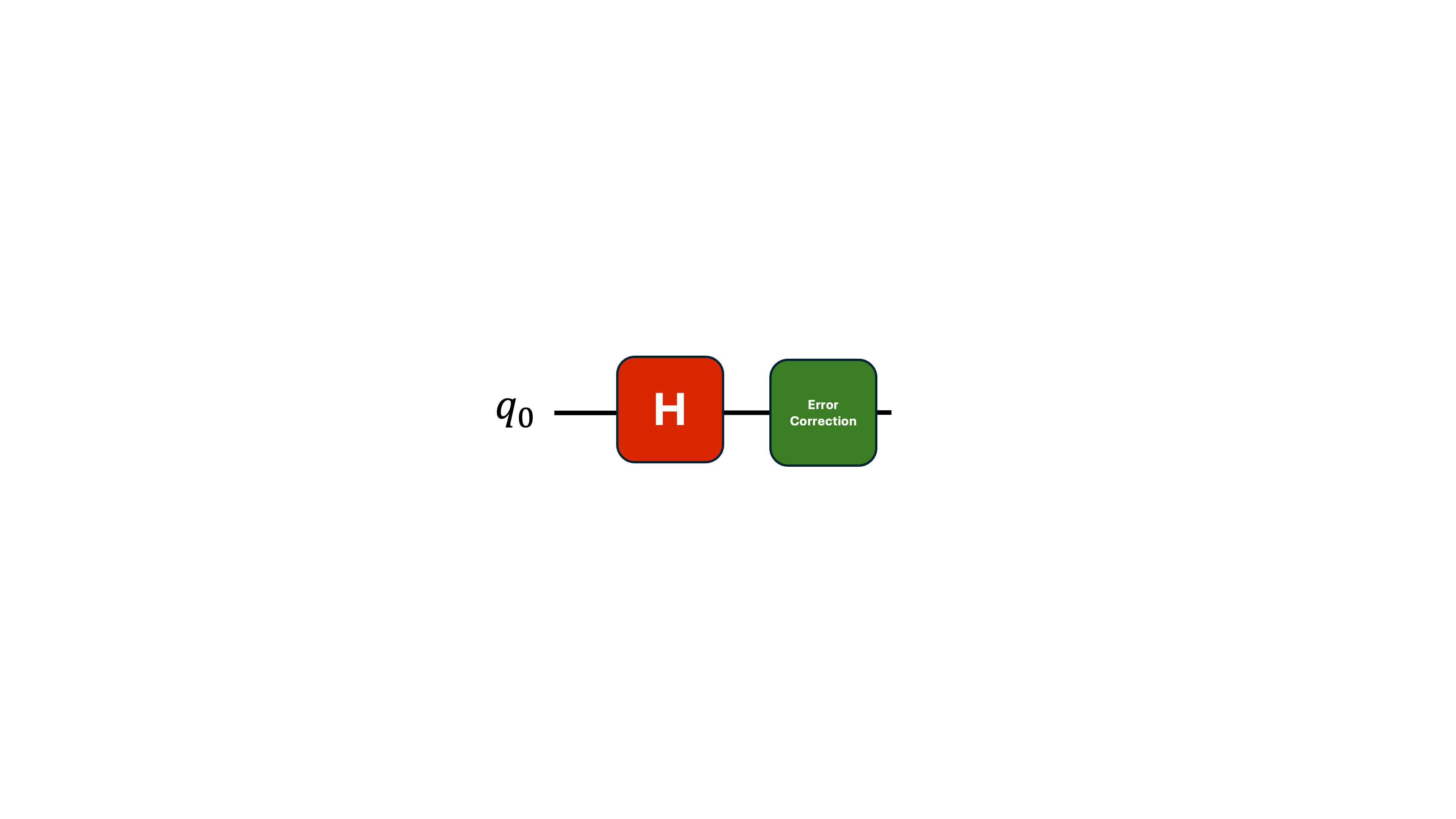
To visualize this, imagine a circuit where both qubits start in |0⟩, and then something in the environment flips one of them.

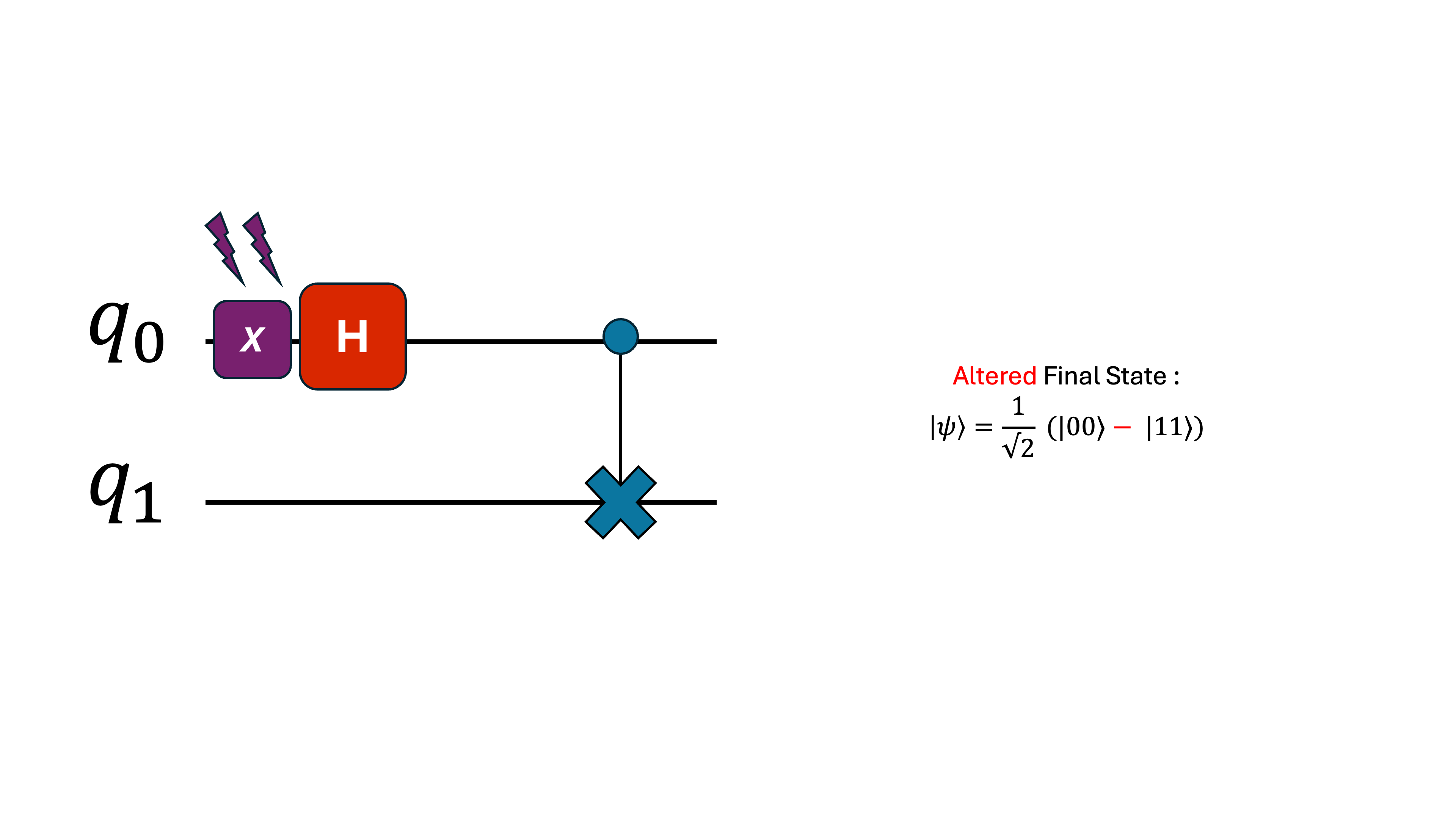
Even a tiny, single-qubit error like this can compound into massive deviation in more complex circuits with many gates and qubits.

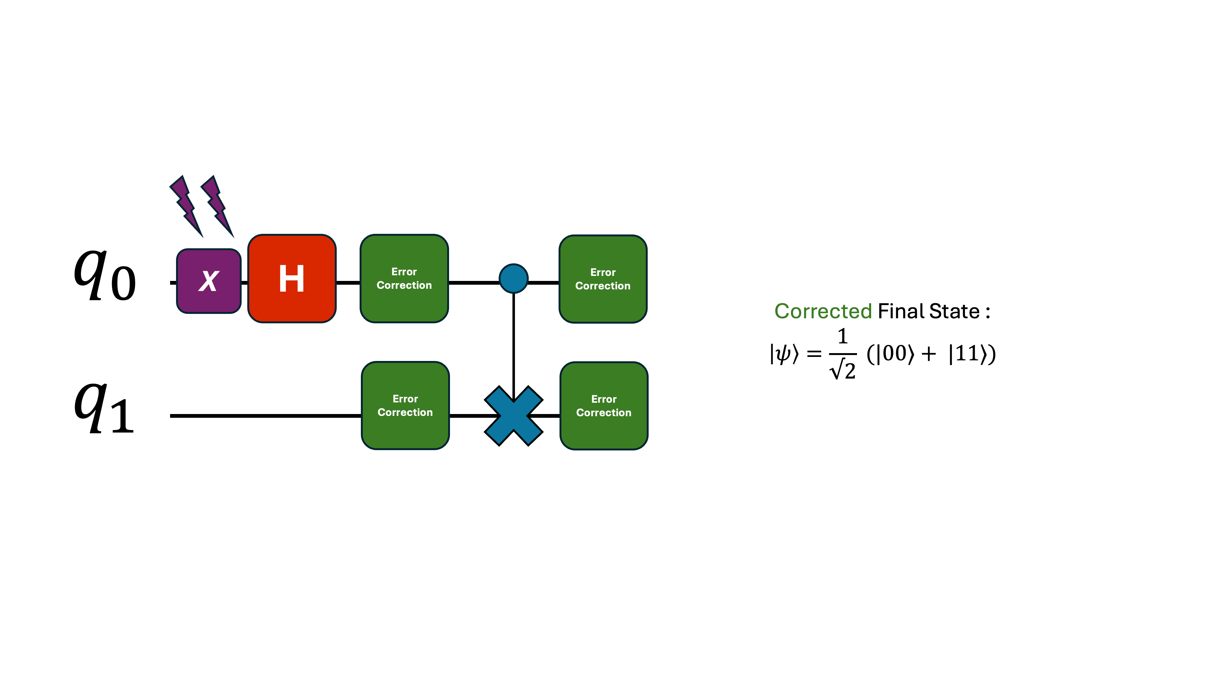
So we introduce an error-correction module that does two things: 1. Detects where the error occurred. 2. Corrects it before it propagates.

What does this error correction module look like?

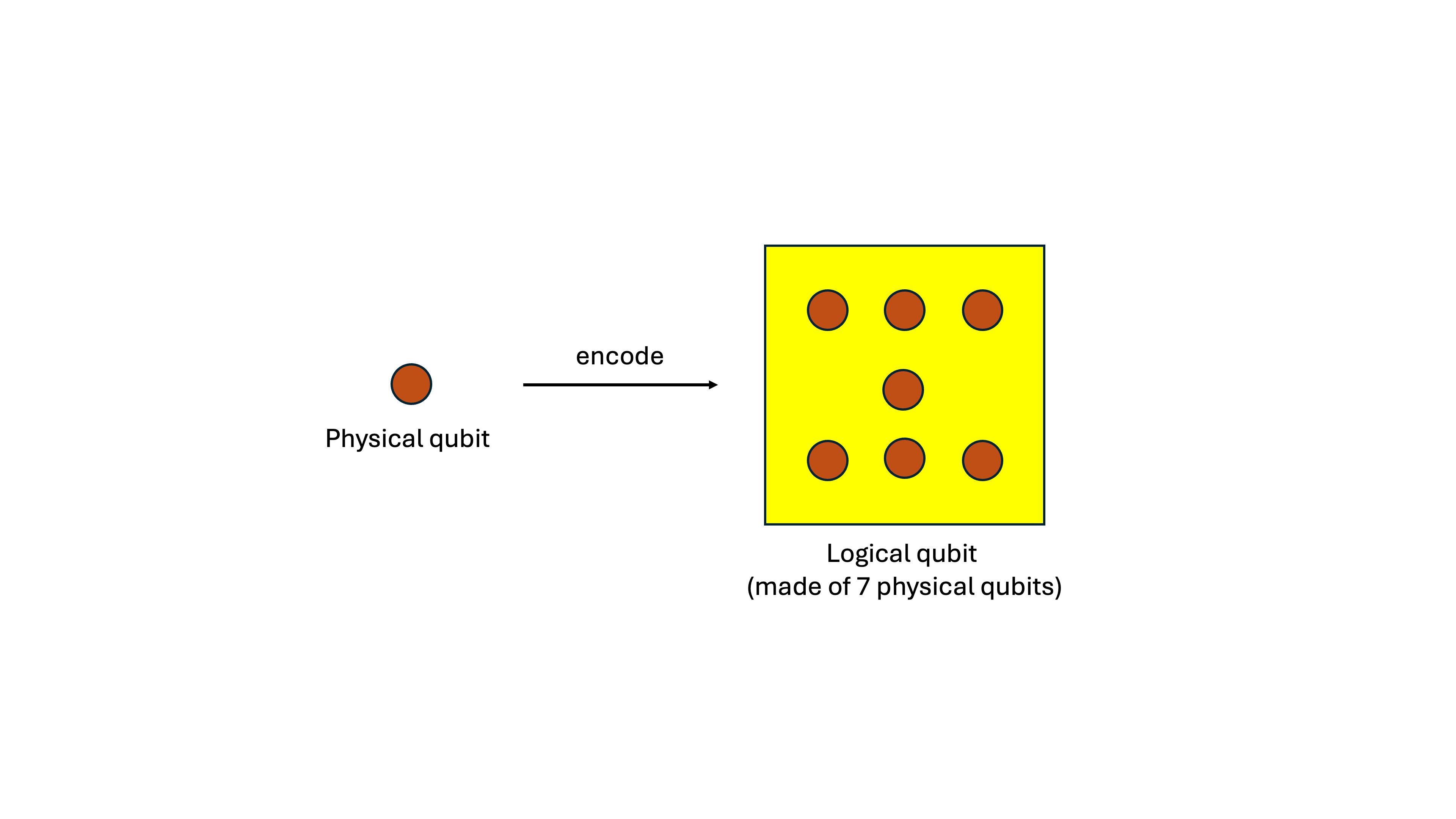
Since a single physical qubit is fragile, we group several noisy qubits together and let them “watch each other’s backs.” That team behaves like one logical qubit—a protected representation of a single unit of information spread across many physical qubits.

If one qubit in the group misbehaves, the others can notice something is wrong.
We detect the mistake.
We correct it.

This logical qubit becomes the basic building block of quantum error correction. We “encode” the information of the qubit we care about across the full group.

Error-correction modules can be designed in many ways, with complexity increasing quickly as you try to handle more types or numbers of errors. For this example, we’ll use a simple scheme (called as the Steane code) that corrects only a single bit-flip error and imagine we want to apply a Hadamard gate on an encoded qubit.

We want to encode the state across 7 data qubits—this is the Steane code’s bit-flip correction circuit. (Don't worry about the details for now - we just need to know it's some protocol that uses 7 + 3 qubits to correct a single bit-flip)

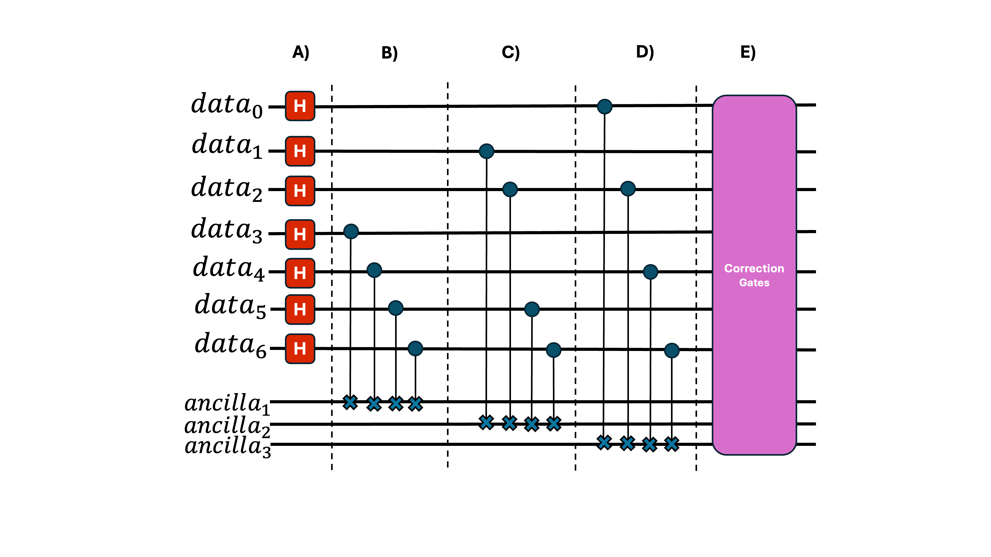
I agree—it looks intimidating at first glance. So let’s zoom into sections A, B, and E.

In the first subsection, we apply our intended Hadamard gate across all data qubits.

In the following subsection, we perform parity checks—tests that determine whether a group of qubits has even or odd parity. These checks place the ancilla qubit into a state that indicates whether an error occurred on the physical qubits.

In the final section, we use the state of the ancilla to decide which correction to apply to the data. Conceptually, this is like an if–else condition: for instance, if data qubit 1 experienced an X error, the pink module can detect that (details outside the scope of this post) and apply an X gate to undo it.

Remember: this simple code handles only one error. Modern error-correction schemes handle multiple simultaneous errors and much richer error types—this is one of the most active areas of research.

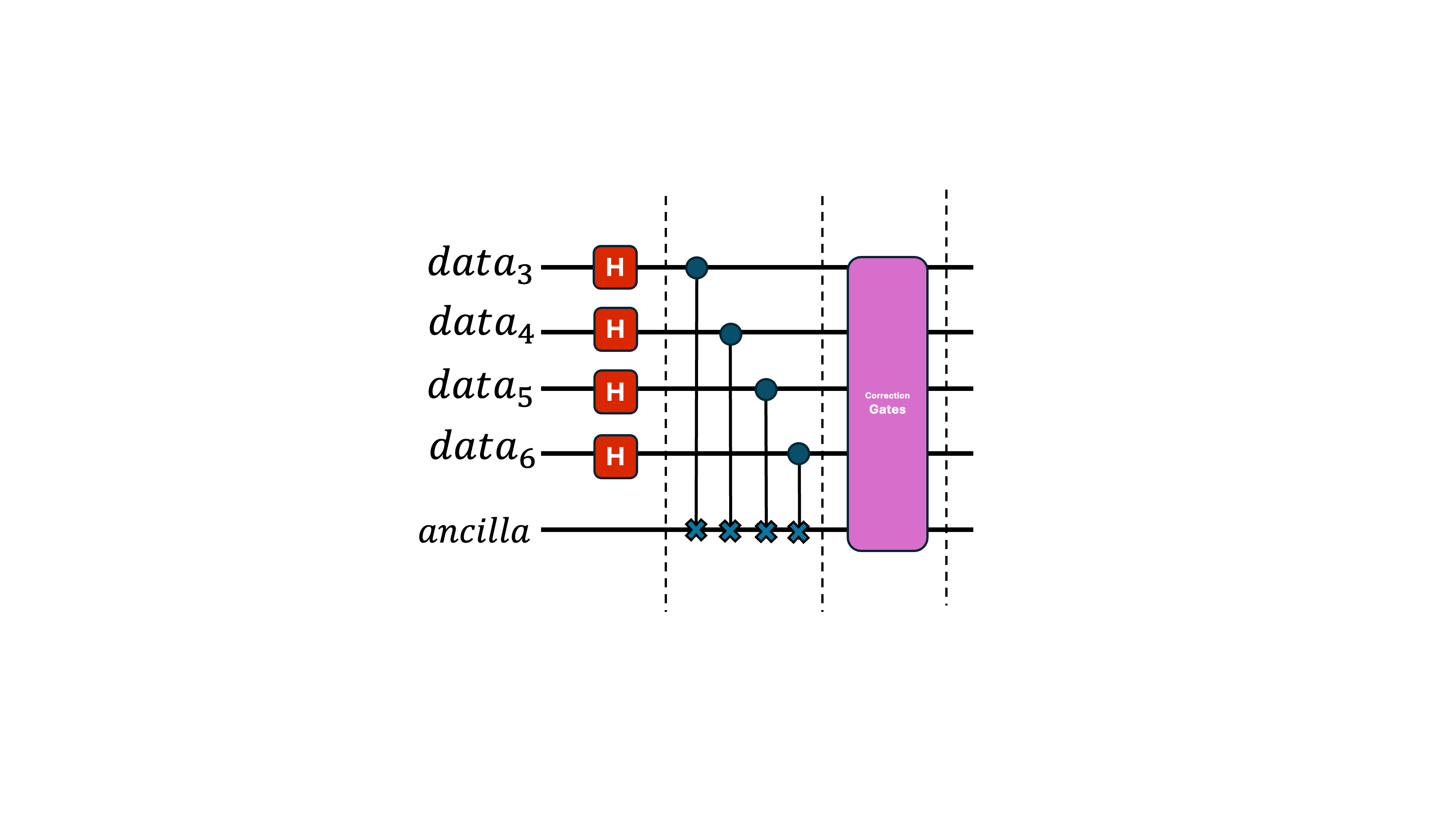
We can also visualize how errors propagate. Imagine the pink module can only correct errors if one or fewer pink bars enter.

What if the Ancilla Qubit Errors?

Alright, I see how we correct an error on a data qubit. But what if the ancilla had an qubit error instead?

Great question—and yes, this can absolutely happen.

So does the same error-correction circuit still work?

Absolutely not.
In fact, the entire error-correction scheme breaks down.

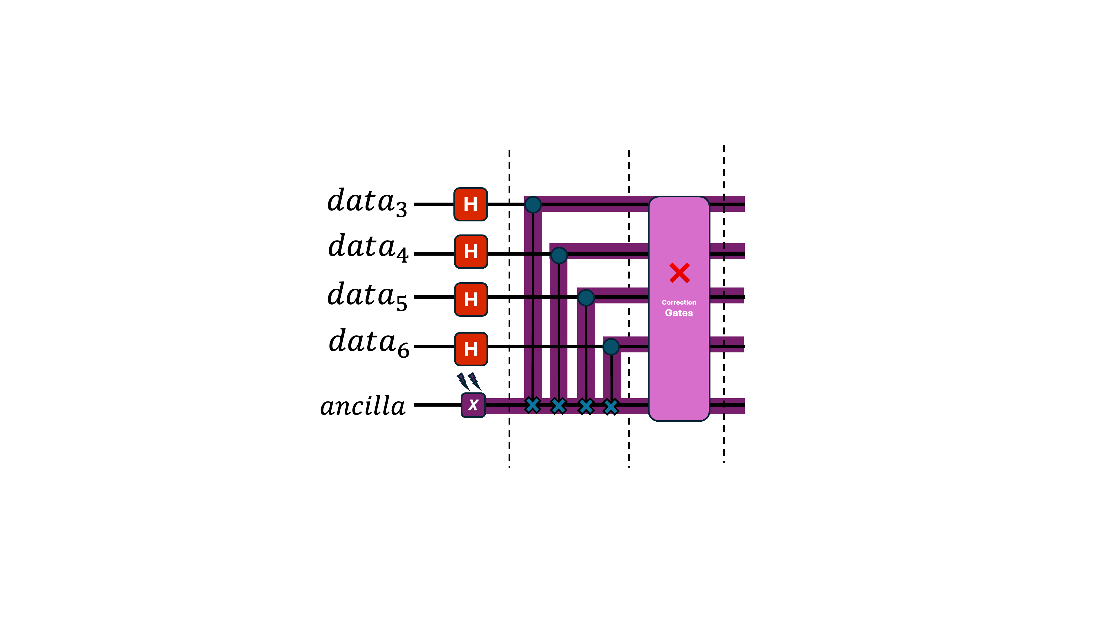
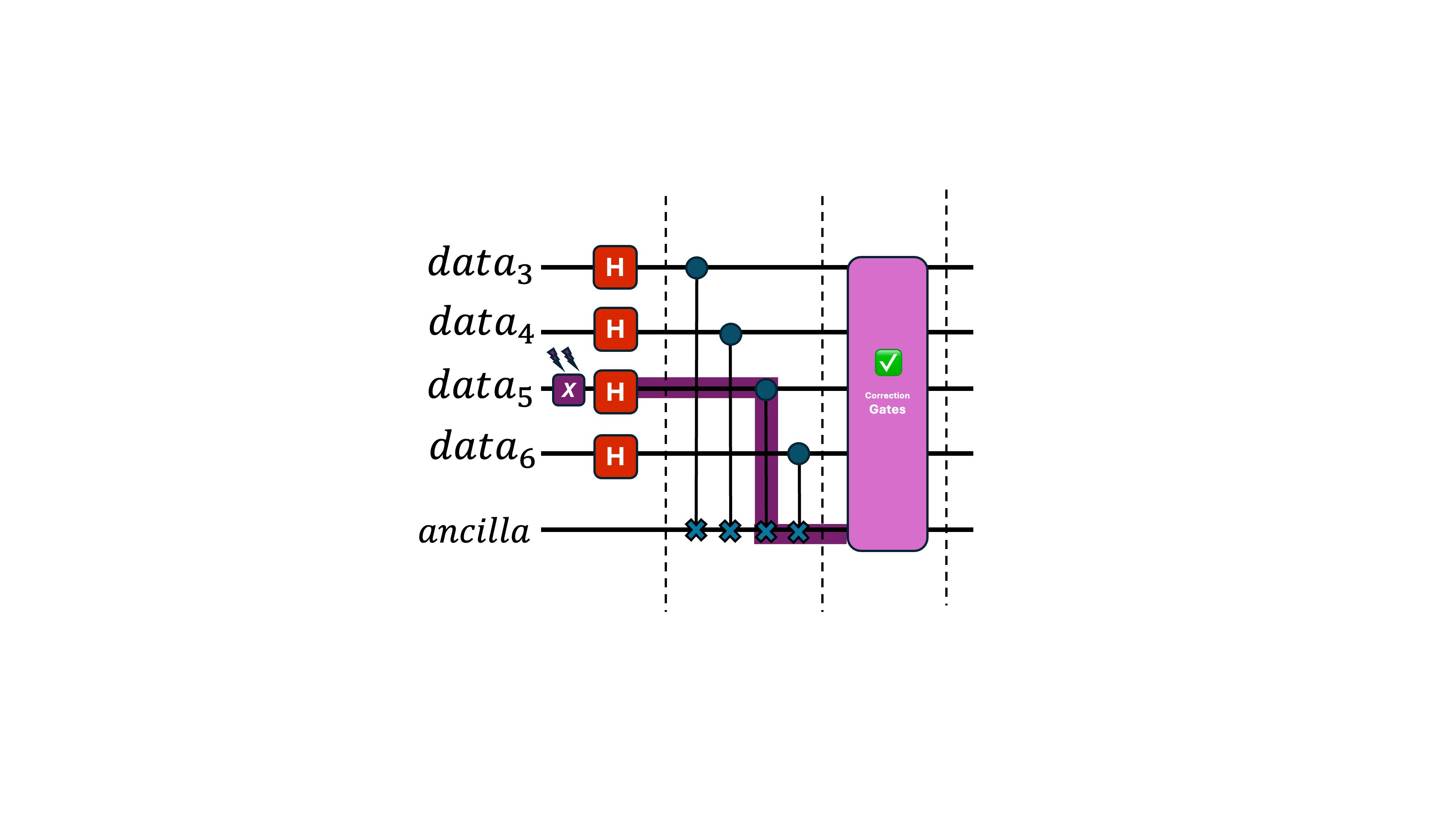
If the ancilla qubit errors, and then interacts with multiple data qubits through gates like CNOT, that single error can spread across the data block. This produces too many errors for the simple pink module to handle, causing the correction to fail completely.

A single fault has now created uncorrectable damage.

How Do We Fix This? Enter Fault Tolerance

Fault tolerance involves protocols designed to ensure that a single physical error cannot spread and create multiple errors that corrupt the logical qubit.

The fix in this example is straightforward:
Use more ancilla qubits.

Instead of using one ancilla as the target of all CNOT gates, we use four ancillas—so each data qubit interacts with only one ancilla. This prevents errors from multiplying. (We also initialize the ancillas in a special state, but that detail isn’t important here.)

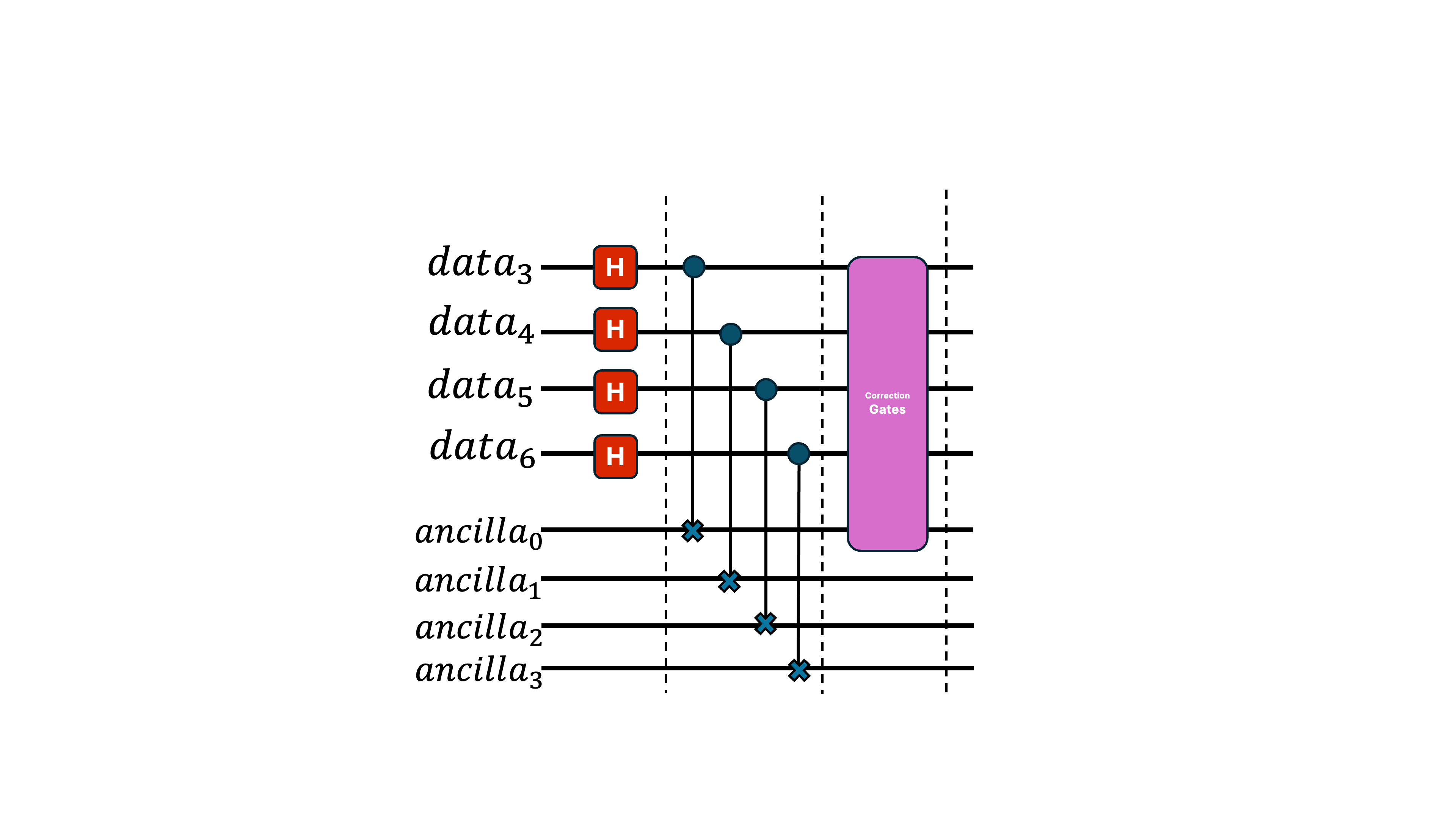
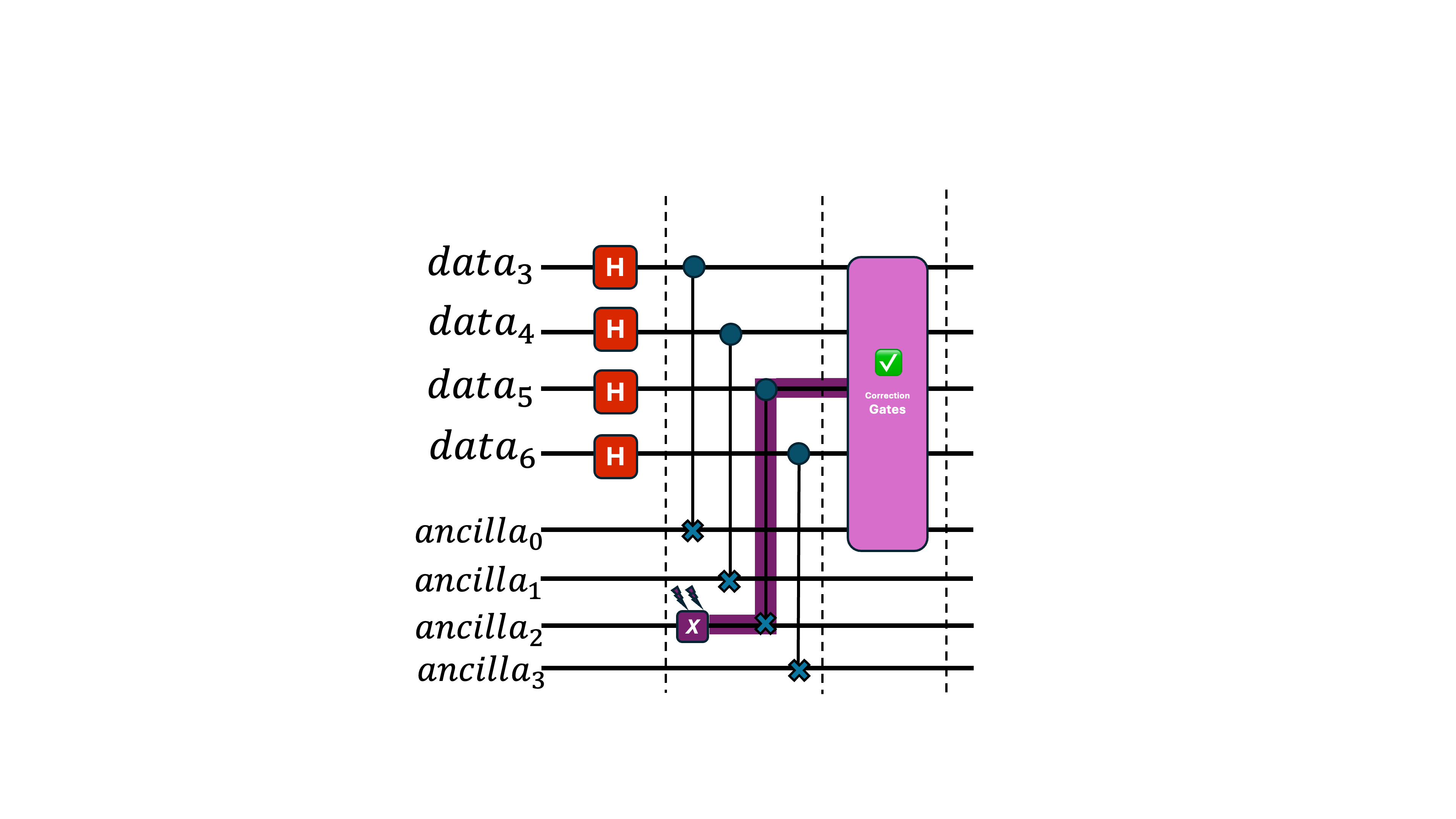
Now, even if one ancilla has an error, it won't propagate uncontrollably, and the correction module can still fix everything properly.

That’s basically it. Hopefully, you have a big-picture idea of the differences between error correction and fault tolerance.

Note: In fact, all three stages—initialization, gates, and measurement—can be and should be performed fault-tolerantly. This ensures the entire computation is protected end-to-end before we even discuss the resource overhead. In this post, we only show fault tolerance applied to error correction. While this post focuses on the fundamental idea behind Fault Tolerance, at the circuit-level, the same concept is applied in different parts of the system that I recommend you read more into.

Conclusion

Before we wrap up, notice how quickly the resource cost grows: even this simple, single-error-correcting example required extra code qubits, ancilla qubits, and additional gates—and making it fault-tolerant added even more overhead. Now imagine a full-scale scheme that can handle any error, at any location, at any time.

The required resources scale fast.

Designing quantum error-correction and fault-tolerant protocols that remain efficient as systems grow is one of the most active and important research challenges in the field today.